Principles of Hierarchical Clustering

These are notes I previously collected and organized. I hope sharing them helps someone understand the logic and principles of hierarchical clustering.

Principles

In a clustering problem, points considered part of one group are either close to one another or share features to some degree. Classifying samples directly by features or indicators after obtaining a dataset is more suitable when business expertise is strong or the indicators are explicit—for example, a hard requirement to group men and women separately. Here I focus on hierarchical clustering.

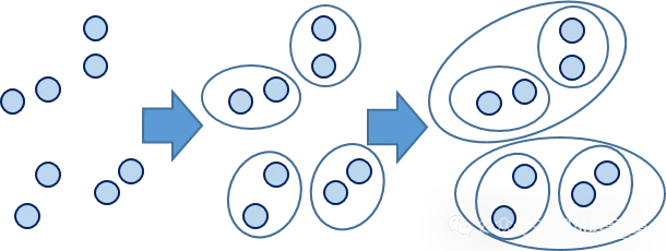
Hierarchical clustering builds clusters at different levels and forms a tree with clusters as nodes, called a clustering diagram. There are two main approaches:

• Bottom-up agglomeration: start with each object as a separate cluster and gradually merge clusters until a stopping condition is met. It is the most common approach and the focus of this article.
• Top-down division: begin with every object in one cluster, then divide it into smaller clusters until a stopping condition is met.

Derivation and distance calculations

Distance

Suppose two observations have attributes represented by vectors. Their distance can be calculated in the following ways:

• Drawbacks of Euclidean distance: it is strongly affected by units, does not account for differences in variable variance, is sensitive to outliers and ignores correlations between indicators. Standardizing or normalizing data before calculating distance can help.
• Drawbacks of Minkowski distance: it depends on the units of indicators and does not consider correlation or relative importance among variables.
• Most inclusive distance: Minkowski distance, since setting q to 1 or 2 gives absolute-value and Euclidean distance, respectively.

Distance between points is straightforward. We commonly use Euclidean distance, based on the right-triangle relationship learned at school—the square root of ab² + bc².

Methods for distances between clusters have evolved. A mainstream approach is average linkage: for two clusters, use the mean of all distances between their points. Its drawback is sensitivity to outliers; median linkage can be used to reduce their influence.

Other common methods include:

• Average linkage: minimize the average distance between samples in pairs of clusters.
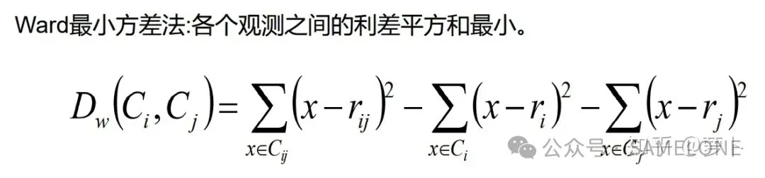
• Ward: minimize the total within-cluster sum of squared deviations. This variance-minimizing optimization resembles the objective in K-means but uses agglomerative hierarchical clustering.
• Maximum or complete linkage: minimize the distance between the farthest samples in pairs of clusters.
• Single linkage: minimize the distance between the nearest samples in pairs of clusters.

• Centroid method: use the distance between two cluster centroids—mean vectors—as the distance between them, similar to the underlying principle of K-means.

The following diagram shows how their results differ, excluding the centroid method:

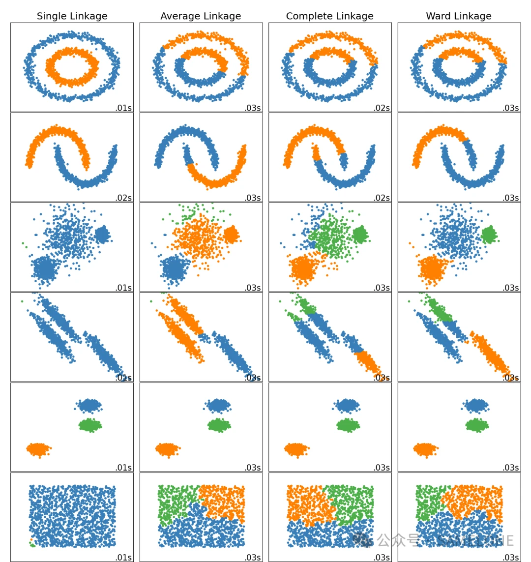
Average linkage and the centroid method are now used less often, in my experience. Ward is commonly chosen because it is less affected by outliers and can perform well even when the distribution is unknown.

Ward's method: theory and example

Ward's method resembles analysis of variance: it uses inter-group distances to determine distances between points, points and clusters, and clusters.

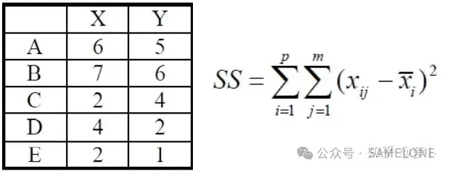
When merged into three clusters—for example AB, CD and E—the combined within-group SS is 1 + 4 + 0 = 5. When two points form a cluster, the within-cluster SS is calculated from the coordinates of one point and the other coordinates in that cluster.

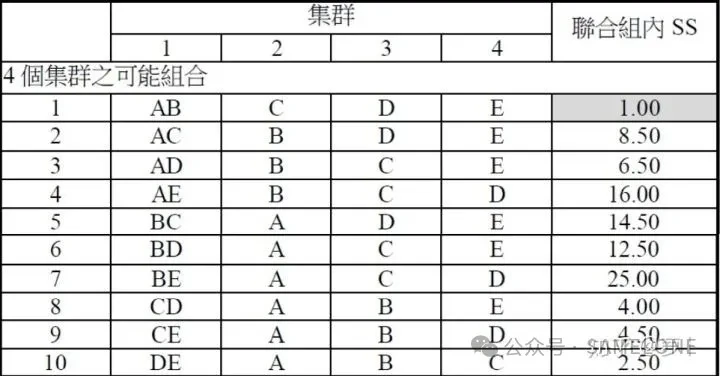
With five points grouped into four clusters, two points are grouped together and the remaining three each form a cluster. There are ten possibilities, shown below:

Likewise, the cases for five points grouped into three, two and one cluster are:

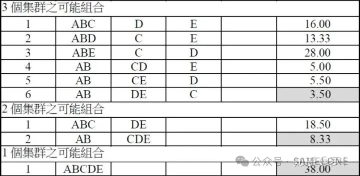
Once two points such as A and B are merged, they take part in later steps as a unit; they are not separated again. From the cases above:

• For four clusters, AB together and the other three points separate gives the lowest SS.
• For three clusters, AB and DE together as separate clusters, with C alone, is best.
• For two clusters, AB and CDE as the two groups is best.
• For one cluster, there is little to analyze.

Notes for a coding project

Before beginning, remember that raw data usually needs preparation:

• Handle missing values.
• Handle extreme outliers.
• Convert categorical variables to dummy variables (0/1 values).
• Avoid an excessive number of categories.

Standardize the data to avoid distance distortions from different units. Statistical methods also have different requirements:

• Decision trees and random forests allow missing values and outliers.
• Clustering and regression models do not support missing values.

Two further questions matter:

1. In clustering, all X variables must be continuous, because distances cannot be calculated directly for categorical variables. For example, distance between people on gender or education level is difficult to calculate, so avoid categorical variables where possible.
2. This does not make categorical variables useless. Cluster using other continuous variables first and then describe the resulting groups statistically. Or use categories to make an initial classification before further clustering, depending on the business need.

For a market research example, suppose a questionnaire investigates “customer needs and attitudes” with the aim of segmenting needs. If many responses are yes/no, combine the answers to multiple questions to create a continuous variable from several categorical variables.

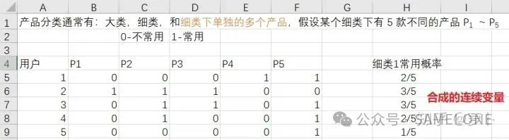
Cosine similarity can also be calculated between categorical variables and used directly as a distance. In any case, categorical variables need treatment in clustering.

Frequently asked questions

Why is a dendrogram unique to hierarchical clustering?

A dendrogram's horizontal axis marks each sample and displays the clustering result. Even with dozens of samples it can become hard to read; with hundreds or thousands, observation is harder still.

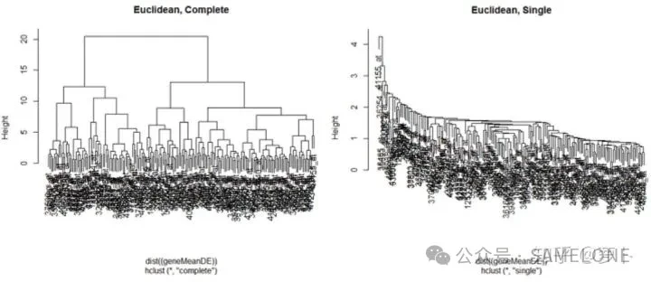
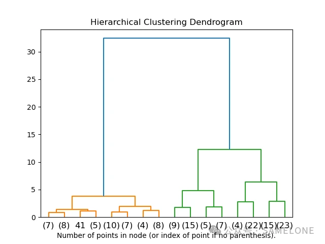
How is a dendrogram built?

Building it represents the clustering process. The tree shows hierarchical relationships between clusters—how far apart they are—and can help determine a suitable number of clusters and see the order in which they were formed. The basic steps are:

1. Calculate the distance between every pair of observations.
2. Merge the two nearest observations, treat them as a unit and calculate their distances to other observations or clusters.
3. Repeat until all observations belong to one cluster.

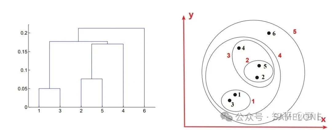
How can the clustering process be read from the tree?

• When two points form one cluster, their lines extend upward from the horizontal axis and meet in a horizontal bar.
• When two clusters merge, lines extend upward from the midpoints of their bars.
• The number of horizontal bars shows how many clustering operations occur as all points become one cluster.

• Bar height indicates merge order; bar width indicates cluster size.

• The whole dendrogram consists of smaller trees, each representing a cluster. A small tree's height is the distance between two points or clusters; the closer they are, the shorter the tree should be.

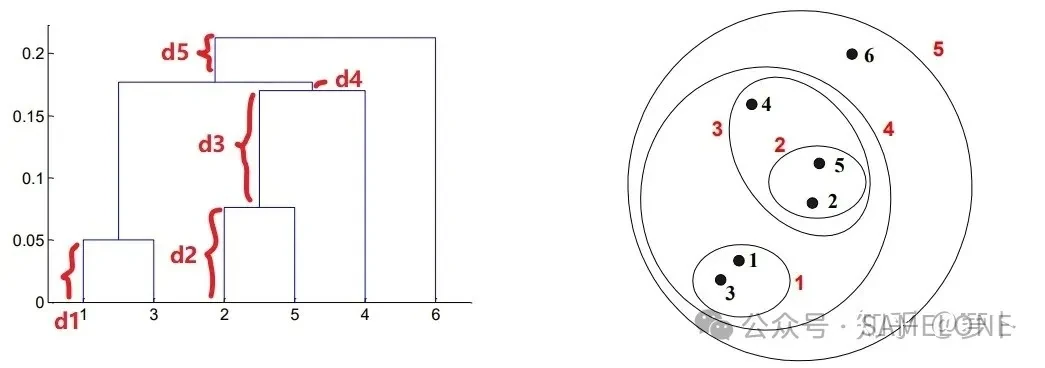
Starting with the smallest height, d1 is the distance between isolated points 1 and 3 in cluster (1,3); d2 is the distance between points 2 and 5 in cluster (2,5). Distances d3, d4 and d5 are not complete tree heights in the same way: they are more like extending branches. d3 extends upward from the midpoint of the (2,5) bar and represents its merge with point 4 to form (2,5,4). Likewise, d4 represents the merge of (2,5,4) with (1,3) to form (1,3,2,5,4); d5 represents that cluster merging with point 6 into the full cluster.

How can the clusters themselves be read from the tree?

A dividing line on the vertical axis can determine how many groups the data is split into.

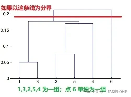
One concern is that three groups—13, 254 and 6—may not be ideal. Tree height represents distance between points; the distance from 4 to cluster 25 is only slightly greater than the distance inside cluster 13, as shown below. Grouping 4 with 25 feels somewhat forced and may cause us to overlook the value of point 4 on its own. It may be better to treat 4 as a separate cluster.